Why Various Distributions Are Appropriate

Why are Weibull, lognormal, and exponential distributions more appropriate than others for modeling failure distributions?

In this article, I want to show you why Weibull, lognormal, and exponential distributions are more appropriate than others for modeling failure distributions. Instead of starting from the explanation of the most used fitting distributions in reliability engineering, I will begin with the analysis of artificial datasets created assuming specific failure behaviors. In other words, I will start from the data and not from the statistical distributions. I think that this approach can help those who deal with this topic for the first time.

Before delving into the topic let’s recall the concept of failure rate and failure probability. These two quantities will be used when elaborating the artificial datasets.

Failure rate is defined as the number of failures in a certain time interval (eq.1)

$$ \lambda(t)=(n(t)-\frac{n(t+\delta t))}{(\delta t\centerdot n(t))} \tag{eq1} $$

Where: 

• $-n(t)-$: number of operational units at time t.
• $- \delta t -$: time interval

The numerator $-n(t) – n(t + \delta t)-$ represents the number of failures occurred in the time interval $- \delta t -$.

Failure probability is defined as the probability that an item fails after a certain time (eq.2). 

$$ R(t)=\frac{n(t)}{n_{0}} \tag{eq2} $$

Where:

• $-n_{0}-$: number of operational units at time t = 0.

In the following I’m going to show four different examples of datasets, They are created assuming different failure behaviors. In all the examples, the number of samples at the beginning of the analysis is n = 10.000 and a unitary time frame is used.

Example 1 – constant failure rate.

For the dataset of failures in Table 1 I’ve assumed a constant failure rate: λ = 0.1.

Table 1. Example 1: constant failure rate. λ = 0.1; Inputs: 

Survival at the beginning of the time interval	Failure rate	Failures	Time interval	Failures (cumulated)	Failure probability
10000	0.1	1000	1	1000	0.10
9000	0.1	900	2	1900	0.19
8100	0.1	810	3	2710	0.27
7290	0.1	729	4	3439	0.34
6561	0.1	656	5	4095	0.41
5905	0.1	590	6	4686	0.47
5314	0.1	531	7	5217	0.52
4783	0.1	478	8	5695	0.57
4305	0.1	430	9	6126	0.61
3874	0.1	387	10	6513	0.65
3487	0.1	349	11	6862	0.69
3138	0.1	314	12	7176	0.72
2824	0.1	282	13	7458	0.75
2542	0.1	254	14	7712	0.77
2288	0.1	229	15	7941	0.79
2059	0.1	206	16	8147	0.81
1853	0.1	185	17	8332	0.83
1668	0.1	167	18	8499	0.85
1501	0.1	150	19	8649	0.86
1351	0.1	135	20	8784	0.88
1216	0.1	122	21	8906	0.89

A constant failure rate implies that in each time interval the quotient between the number of failures at the end of the time interval and the surviving items at the beginning of the time interval is constant (Figure 1a). Does the assumption of constant failure rate apply to any failure-related event? Yes, if failure is caused by random phenomena. Examples are: flat tire due to a sharp object, electronics failure due to power surge, electronics failure due to cosmic radiation. In these cases, the failure rate doesn’t change with time. In more simple words, the failure rate related to a flat tire due to a sharp object does not depend on the tire age.

Figure 1b shows the number of failures over time. Data points shown in Figure 1b can be well fitted by an exponential distribution. Alternatively, the Weibull distribution with shape parameter β = 1 can be applied.

Example 2 – linearly increasing failure rate.

For the dataset in Table 2, I’ve assumed a linearly increasing failure rate (λ_i+1 = λ_i + 0.04; λ₀ = 0.04). 

Table 2. Example 2: increasing failure rate: λ_i+1 = λ_i + 0.04; λ₀ = 0.04.

Survival at the beginning of the time interval	Failure rate	Failures	Time interval	Failures (cumulated)	Failure probability
10000	0.04	400	1	400	0.04
9600	0.08	768	2	1168	0.12
8832	0.12	1060	3	2228	0.22
7772	0.16	1244	4	3471	0.35
6529	0.20	1306	5	4777	0.48
5223	0.24	1253	6	6031	0.60
3969	0.28	1111	7	7142	0.71
2858	0.32	915	8	8057	0.81
1943	0.36	700	9	8756	0.88
1244	0.40	498	10	9254	0.93
746	0.44	328	11	9582	0.96
418	0.48	201	12	9783	0.98
217	0.52	113	13	9896	0.99
104	0.56	58	14	9954	1.00
46	0.60	28	15	9982	1.00
18	0.64	12	16	9993	1.00
7	0.68	4	17	9998	1.00
2	0.72	2	18	9999	1.00
1	0.76	0	19	10000	1.00
0	0.80	0	20	10000	1.00

Does this assumption apply to any failure-related event? Yes, if failure is caused by wear-out mechanisms. Wear-out mechanisms are time dependent. That means the older the product, the higher the number of failures for the same time interval will be. Examples of wear-out mechanisms are: fatigue, wear, creep, thermal ageing. Plotting failures over time results in a different shape when compared to example 1 (Figure 2b). Failures initially increase but with decreasing number of alive items they start to decrease until all items have failed.

In this case, positively skewed distributions such as Weibull or lognormal distribution can be used for fitting failures.

Example 3 – linearly decreasing failure rate.

For the dataset in Table 3, I’ve assumed a linearly decreasing failure rate (λ_i+1 = λ_i – 0.01; λ₀ = 0.05).  

Table 3. Example 3: linearly decreasing failure rate: λ_i+1 = λ_i – 0.01; λ₀ = 0.05.

Survival at the beginning of the time interval	Failure rate	Failures	Time interval	Failures (cumulated)	Failure probability
10000	0.050	500	1	500	0.05
9500	0.049	466	2	966	0.10
9035	0.048	434	3	1399	0.14
8601	0.047	404	4	1803	0.18
8197	0.046	377	5	2180	0.22
7820	0.045	352	6	2532	0.25
7468	0.044	329	7	2861	0.29
7139	0.043	307	8	3168	0.32
6832	0.042	287	9	3455	0.35
6545	0.041	268	10	3723	0.37
6277	0.040	251	11	3974	0.40
6026	0.039	235	12	4209	0.42
5791	0.038	220	13	4429	0.44
5571	0.037	206	14	4635	0.46
5365	0.036	193	15	4829	0.48
5171	0.035	181	16	5010	0.50
4990	0.034	170	17	5179	0.52
4821	0.033	159	18	5338	0.53
4662	0.032	149	19	5487	0.55

Failures decrease over time from the beginning. Does this assumption apply to any failure-related event? Yes, we might observe a decreasing failure rate when failures occur due to manufacturing-related issues. In such cases, product fail just after installation. Since they are just a fraction (hopefully!) of the entire population, as soon as they fail, the chance of failure for the rest of population decreases over time.

In this case, a Weibull distribution with shape parameter β < 1can be used for fitting failures.

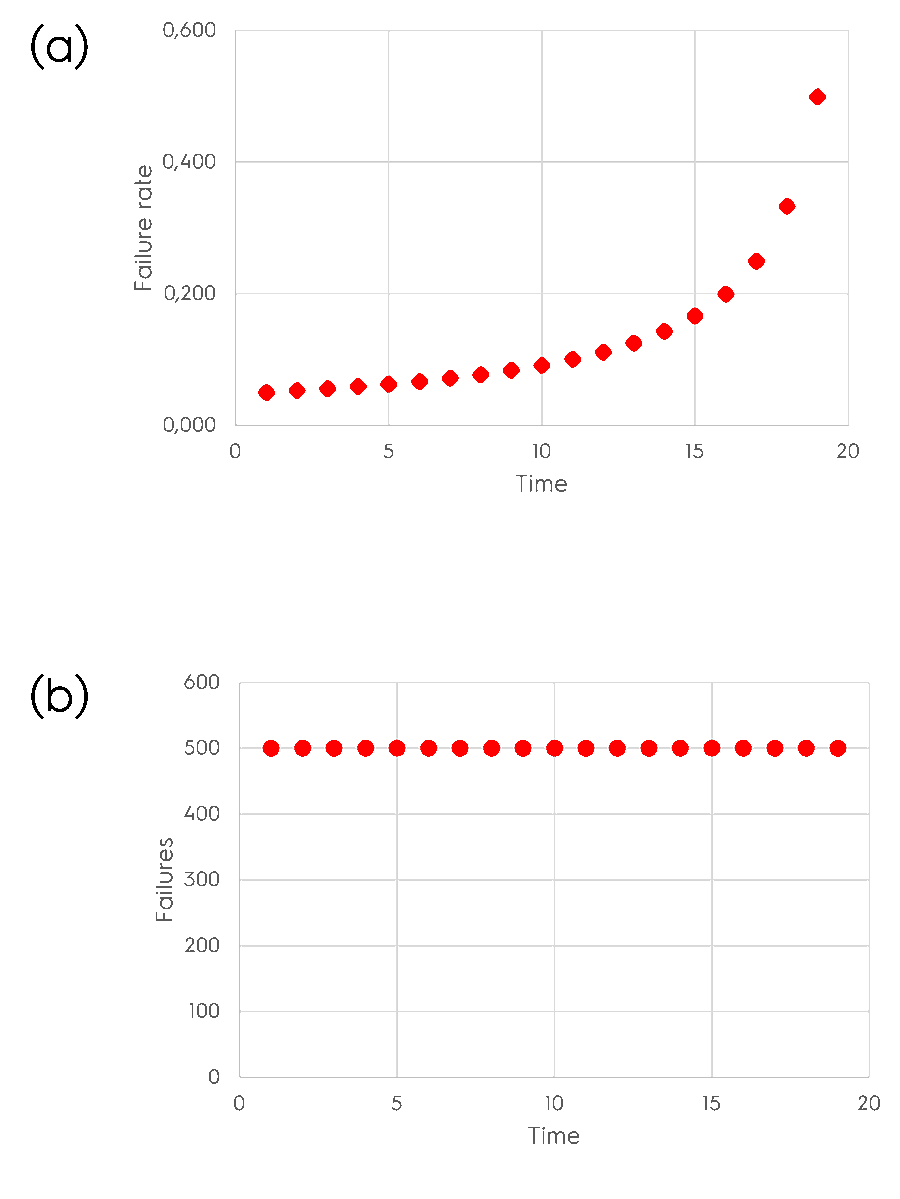
Example 4 – constant number of failures over time.

In this last example, I’ve assumed that the number of failures is constant over time (failures = 500). 

Table 4. Example 4: constant number of failures over time. Failures = 500.

Survival at the beginning of the time interval	Failure rate	Failures	Time interval	Failures (cumulated)	Failure probability
10000	0.050	500	1	500	0.05
9500	0.053	500	2	1000	0.10
9000	0.056	500	3	1500	0.15
8500	0.059	500	4	2000	0.20
8000	0.063	500	5	2500	0.25
7500	0.067	500	6	3000	0.30
7000	0.071	500	7	3500	0.35
6500	0.077	500	8	4000	0.40
6000	0.083	500	9	4500	0.45
5500	0.091	500	10	5000	0.50
5000	0.100	500	11	5500	0.55
4500	0.111	500	12	6000	0.60
4000	0.125	500	13	6500	0.65
3500	0.143	500	14	7000	0.70
3000	0.167	500	15	7500	0.75
2500	0.200	500	16	8000	0.80
2000	0.250	500	17	8500	0.85
1500	0.333	500	18	9000	0.90
1000	0.500	500	19	9500	0.95

Despite the number of survivals decreases over time, the number of failures doesn’t. Do we find something similar in nature? Honestly speaking, we don’t. For this reason, we won’t deal with modeling data shown in Figure 4.

Conclusions

We have seen that different fitting distributions apply to different failure-related phenomena. Exponential, Weibull, and lognormal distributions are the most used functions since they can model failures in different but realistic situations.