
Rupert Miller said, “Surprisingly, no efficiency comparison of the sample distribution function with the mles (maximum likelihood estimators) appears to have been reported in the literature.” (Statistical “efficiency” measures how close an estimator’s sample variance is to its Cramer-Rao lower bound.) In “What Price Kaplan-Meier?” Miller compares the nonparametric Kaplan-Meier reliability estimator with mles for exponential, Weibull, and gamma distributions.
This report compares the bias, efficiency, and robustness of the Kaplan-Meier reliability estimator from grouped failure counts (grouped life data) with the nonparametric maximum likelihood reliability estimator from ships (periodic sales, installed base, cohorts, etc.) and returns (periodic complaints, failures, repairs, replacement, spares sales, etc.) counts, estimator vs. estimator and population vs. sample.
Ships and Returns Counts?
Ships and returns counts, (sums of period returns in bottom row of table 1) are statistically sufficient to make nonparametric reliability and failure rate function estimates. Ships and returns counts are modeled as inputs and outputs of M/G/infinity self-service systems. The output of an M/G/infinity self-service system is a Poisson process with rate λG(t), where λ is the Poisson process input rate and G(t) represents the service time distribution function, one minus the reliability function. If λG(t) is nondecreasing, then majorization yields the nonparametric maximum likelihood estimator of the reliability function R(t)=1-G(t) [George and Agrawal].
Our article was published in the Naval Research Logistics Quarterly (NRLQ). It was about estimating service time distribution G(t) from input and output counts of an M/G/infinity self-service system with Poisson input process. Seymour Selig, then editor of NRLQ, asked me, “What is the precision of the estimator?” (the nonparametric maximum likelihood estimator from ships and returns counts) I didn’t know, but I knew how to find out.
The hypothesis of stationary Poisson process input to an M/G/infinity self-service life system is testable. Goodness-of-fit tests could be used test the Poisson assumption. The usual test is based on the observations of the times between the individual units shipped.
The nonstationary-Poisson-input M(t)/G/infinity conditions for existence of the nonparametric maximum likelihood estimator of G(t) are in an unpublished article [George, 1994] and in a presentation on the rate of convergence of maximum likelihood estimators [Wellner, Nemirovskll et al.].
The hypothesis of a nonstationary Poisson process M(t) inputs to an M(t)/G/infinity system is not fully testable, The Poisson assumption is testable, if not too nonstationary. Use the Z-test (approximate normal distribution) of (ΔM(t)-E[ΔM(t)])/√E[ΔM(t)], where ΔM(t) is number of inputs around time t, bootstrapped with different interval widths.) However, the hypothesis of independent increments is not testable unless you have multiple sample realizations from the Poisson ships process for the times t under observation. Period inputs such as ships counts provides a sample of size one for each time increment, so the assumption of nonstationary Poisson ships is not fully testable; i.e., the assumption of nonstationary Poisson is hard to refute.
Sample Bias?
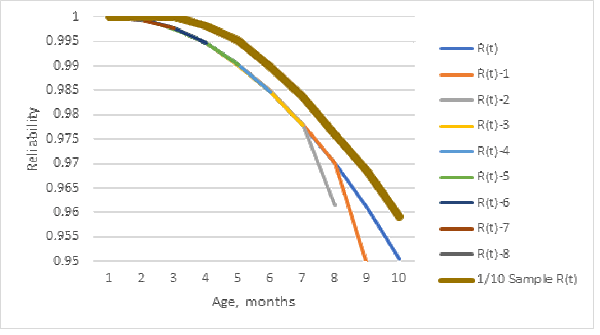
Sample bias depends on how a sample is selected and which data is used: grouped failure counts [https://en.wikipedia.org/wiki/Kaplan%E2%80%93Meier_estimator] or ships and returns counts. Figure 1 shows the population and 1/10 sample (table 1) Kaplan-Meier reliability estimates. The bold line is the 1/10 sample Kaplan-Meier reliability estimate from grouped failure data. The 1/10 sample Kaplan-Meier reliability estimate is biased higher compared with population reliability estimator!
“Well Duh!” you may say. A sample does not contain as much information as the population from which the sample is taken. In reliability statistics, sample and population data may be censored. With reliable products, there may not be very many failures. A sample may not even have failures. I checked several other Nevada table data sets, and dividing counts by 10 and rounding off often resulted in zero failures.
Table 1. Part of the Nevada table 1/10 data sample from the 10-month table in [http://www.weibull.com/hotwire/issue119/relbasics119.htm]. The bottom row lists monthly returns regardless of which ships cohort they came from.
| Week | Ships | Mar-10 | Apr-10 | May-10 | Jun-10 | Jul-10 | Etc. |
| Mar-10 | 162 | 0 | 0 | 0 | 1 | 1 | 1 |
| Apr-10 | 372 | 0 | 0 | 1 | 1 | 2 | |
| May-10 | 132 | 0 | 0 | 0 | 0 | ||
| Jun-10 | 360 | 0 | 0 | 1 | |||
| Jul-10 | 330 | 0 | 0 | ||||
| Etc. | |||||||
| Returns | 0 | 0 | 0 | 2 | 2 | 4 |
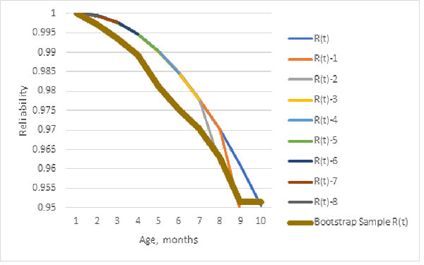
Dividing the population Nevada table entries by 10 Is not a random sample, but it illustrates sample bias. Figure 2 shows that a bootstrap sample (resampling from the population reliability estimate [https://en.wikipedia.org/wiki/Bootstrapping_(statistics)]) gives the opposite bias, less reliability. The bootstrap resamples, from the table 1 ships/10, failure counts simulated from the population Kaplan-Meier population reliability estimate. Using ships/10 with population Kaplan-Meier reliability estimate could explain why the bootstrap sample reliability estimate is biased for lower reliability than the population Kaplan-Meier reliability estimate from which the bootstrap samples are computed. (I recomputed the bootstrap sample estimates many times and the result was usually similar to figure 2.)
Furthermore, the sample Kaplan-Meier estimator is more biased than the maximum likelihood estimator from the same 1/10 sample’s ships and returns counts! This occurred for the Nevada table of 10 months of data (in the previous article about uncertainty [George 2022]), divided by 10 and rounded off to integers (table 1).
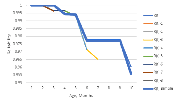
Figure 3 shows that the 1/10 sample reliability estimate, from ships and returns counts, is about the same as the population estimates. The bias of the reliability estimator from ships and returns counts appears negligible, because sampling returns, sums of grouped life data, are less likely to be rounded off to zero than individual months’ grouped failure counts by cohort in the body of the Nevada table.
Use the nonparametric maximum likelihood estimator from sample or population ships and returns counts, unless you already have population life data by individuals or grouped population life data (failure counts) as in a Nevada table. The Kaplan-Meier reliability estimator from a sample of grouped life data could be biased!
Sample Standard Deviation?
Estimator variance or standard measures reliability uncertainty. It is beginning to be accounted for in reliability based design [Coit and Jin, Shi and Shen, Wang et al.]. This report compares the standard deviations of sample estimators vs. population estimators, and compares the standard deviations of the Kaplan-Meier estimator from grouped failure counts vs. the maximum likelihood estimator from ships and returns counts. The standard deviations are the square roots of Cramer-Rao lower bounds on variances, the asymptotic variances of population maximum likelihood estimates [Borgan, https://en.wikipedia.org/wiki/Cram%C3%A9r%E2%80%93Rao_bound].
Greenwood’s variance formula for the variance of the Kaplan-Meier reliability function estimator is the asymptotic Cramer-Rao lower bound (table 2 and figure 4). It is the reliability function R(t) squared times the sum of Deaths/(At Risk*(At Risk-Deaths)) summed over months, R(t)2*∑D(s)/(Y(s)*(Y(s)-D(s)), s=1,2,…,t. Surprise! Dividing deaths D(s) and numbers at risk Y(s) by 10 increases the standard deviations (table 2 and figure 3) by a factor of the square root of 10!
Table 2. Standard deviations (Greenwood) of population and 1/10 sample Kaplan-Meier reliability estimates.
| Age | Sample Stdev | Population Stdev |
| 1 | 0 | 0 |
| 2 | 0 | 0.0001 |
| 3 | 0.0009 | 0.0003 |
| 4 | 0.0016 | 0.0005 |
| 5 | 0.0025 | 0.0008 |
| 6 | 0.0032 | 0.0010 |
| 7 | 0.0042 | 0.0013 |
| 8 | 0.0054 | 0.0017 |
| 9 | 0.0068 | 0.0021 |
| 10 | 0.0110 | 0.0033 |

Sample Efficiency?
Statistical efficiency refers to how close an estimator’s sample variance is to its Cramer-Rao lower bound (CRLB). The CRLB on the reliability estimator variance-covariance matrix is minus the inverse of (the expected value of) the second derivative matrix of the log likelihood function (aka Fisher Information matrix). Maximum likelihood estimators achieve the CRLB asymptotically, under some conditions. Columns two and three of table 3 are the CRLB standard deviations of the maximum likelihood reliability function estimates from the ships of table 1 and returns (bottom row of table 1). The last two columns of table 3 are the standard deviations of the Kaplan-Meier reliability function estimates from 1/10 sample and population data. I added the standard deviations for R(4), reliability at age 4 months, for comparison.
The alternative population estimators’ standard deviations are comparable even though grouped life data (Nevada table) contains more information than ships and returns counts. Their sample standard deviations are of same order of magnitude although the standard deviation of the 1/10 sample ships and returns is greater. There is no reason to collect samples of ships and returns, except to compare their reliability estimates by source or customer. Time and cost motivate samples of ships and grouped failure counts if you want the Kaplan-Meier reliability estimate. Is the difference worth the cost of a sample of grouped failure counts, when population ships and returns are required by Generally Accepted Accounting Principles (GAAP)?
Table 3. The standard deviations and entropies of sample and population reliability estimates from ships and returns counts (columns 2 and 3) vs. grouped life data (columns 4 and 5, from previous article and from monthly returns in the bottom row of table 1). The CRLB sample standard deviation was indeterminate, because there were no failures in the first three age intervals. The fourth standard deviation is the binomial sample standard deviation for the reliability estimate 1-2/1026=0.998 where there were 2 failures and 1026 is the sum of the first four months of ships in table 1.
| Age | Sample Stdev | Pop Stdev | K-M Sample | K-M Pop. Stdev |
| 1 | Indeterm. | 0.000257 | 0 | 0 |
| 2 | Indeterm. | 0.000257 | 0 | 0.0001 |
| 3 | Indeterm. | 0.000363 | 0.0009 | 0.0003 |
| 4 | 0.00138 | 0.000514 | 0.0016 | 0.0005 |
| Etc. | ||||
| Entropy | 0.1829 | 0.1748 | 0.2606 | 0.2954 |
The maximum likelihood population standard deviations in column three “Pop Stdev” are not same as in previous article [George 2022]. I made a correction and added the standard deviation for age 4 months, for comparison with column five “K-M Pop Stdev”. The population standard deviations in columns three and five, maximum likelihood from ships and returns vs. K-M grouped life data, are close despite the K-M grouped life data has more information than ships and returns counts. (The sample standard deviations of reliability estimators from ships and returns counts are in included in table 3 only for comparison with the Kaplan-Meier reliability estimator from the same sample.)
The entropy values in the bottom row show there is more information in grouped life data than in ships and returns, sample or population. It is contrary that the sample entropy from a 1/10 sample of ships and returns is a little more than from the population of ships and returns.
Please recognize that ships and returns counts are population data, from data required by GAAP. There won’t be any more ships and returns counts until the next accounting reporting period. Don’t estimate reliability from samples of ships and returns counts when you have population ships and returns counts.
Confidence Bands?
Don’t believe the confidence bands on Kaplan-Meier reliability estimates at the bottom of Non-Parametric Life Data Analysis – ReliaWiki. They’re confidence limits valid at one age, based on Greenwood’s variance estimate and normal distribution statistics; they don’t mean the entire reliability function estimate will lie within the confidence bands for 95% of the ages. Hall-Wellner confidence bands do [Hall and Wellner]. They use the Cramer-Rao lower bounds on the variance-covariance matrix of estimators.
The asymptotic distributions of maximum likelihood estimators are multivariate normal distributions, so the variance-covariance matrix should be used to construct approximate (asymptotic) confidence bands on reliability or actuarial failure rate function estimates, for confidence or tolerance limits on actuarial forecasts.
Robustness?
Robustness of estimators usually means insensitivity to outliers. However, if data is censored, robustness also includes insensitivity to the distribution(s) of censoring times or their distribution if random. Grouped failure counts in a Nevada table (table 1) are censored by the fact that the oldest cohort is 10 months old, the second oldest cohort is 9 months old, etc. The robustness of the Kaplan-Meier estimator is known [Huber].
Figure 5 and table 5 compare the reliability estimates from the original sample of Nevada table (table 1) as if it were uncensored vs. censored grouped failure counts (table 4). Figure 5 shows the maximum likelihood estimator from censored ships and returns (R(t) S & R) has same hitch as in figure 3. Table 5 compares the entropy (information) in the reliability estimates. Censoring loses some information, but figure 5 shows it doesn’t bias the reliability estimates, unless censoring wipes out the failure counts.
Table 4. Table 1 data censored by an exponential distribution with mean 1000 months.
| Week | Ships | Mar-10 | Apr-10 | May-10 | Jun-10 | Jul-10 | Etc. |
| Mar-10 | 162 | 0 | 0 | 0 | 1 | 1 | 0 |
| Apr-10 | 372 | 0 | 0 | 0 | 2 | 1 | |
| May-10 | 132 | 0 | 1 | 1 | 1 | ||
| Jun-10 | 360 | 0 | 0 | 0 | |||
| Jul-10 | 330 | 0 | 0 | ||||
| Etc. | |||||||
| Returns | 0 | 0 | 0 | 2 | 4 | 2 |
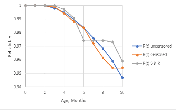
Table 5. Entropies of alternative estimates from sample uncensored and censored with an exponential distribution with mean 1000 periods. Censored entropy values are the averages of 10 simulations.
| Uncensored | K-M censored | S & R censored |
| -0.26058 | -0.24738 | -0.21002 |
Is Grouped Failure Data for Kaplan-Meier Estimates Necessary?
Which should you spend money and time on: improving reliability or reducing uncertainty? Reliability vs. uncertainty decisions should consider risk, the expected costs of whatever decisions you might make on improving reliability or on reducing uncertainty. Improving reliability could reduce warranty reserves, warranty costs, warranty extensions, and recalls. Reducing uncertainty could save money wasted on warranty reserves, service, unnecessary maintenance, and obsolescent spares inventory.
When I worked for Apple Computer I estimated the age-specific field reliability of all computer products and their service parts from product sales, bills of materials, and parts’ returns counts.
I asked Mike, the Apple Service Department accountant, if he wanted help estimating warranty reserves based on the field reliability of Apple products and their service parts? He replied, “No thanks. We already do that based on last year’s warranty reserves, costs, and sales.” I asked him what if you’re wrong? He said, “We just take a charge or a credit depending on actual warranty costs.” Extrapolating time series is like driving by looking backward. Forecasting based on observed field reliability is like driving by looking ahead, because reliability drives the demands for warranty returns or service parts [Buczkowski, Kulkarni]. I wondered what Apple could have done with money squirreled away in warranty reserves?
I wrote a computer program for service providers to forecast spare parts’ demands and recommend stock levels based on service providers’ installed base. When service providers used my computer program to estimate spares stock levels, they found that they had been required, in the past, by Apple, to buy spare parts that had become obsolescent. I was put in charge of buying back $36,000,000 of obsolescent spare parts and distributing the charges over three calendar quarters. That used to be a lot of money wasted (in 1992) by guessing instead of using field reliability to recommend spares stocks. Parts were crushed.
Conclusions?
The Kaplan-Meier estimate, from a sample of grouped failure counts, could be biased, depending on how you take the sample. The sample Kaplan-Meier estimate also has about the same standard deviation as the nonparametric maximum likelihood estimate from population ships and returns counts! These observations on one data set may not generalize, but why take a sample of life data when the population estimator from ships and returns counts has smaller standard deviation? Use the Kaplan-Meier reliability estimator only if you can afford the cost of tracking every product and service part in the installed base by name or serial number from sale or shipment to end of life or suspension.
The standard deviations of the Kaplan-Meier population estimates are less than those from the maximum likelihood estimates, from population ships and returns, but the difference diminishes with age t. The entropy (information) in the Kaplan-Meier estimator is greater, because the Nevada table contains grouped failure counts by cohort. Period returns counts could have come from any earlier ships cohorts.
Unsurprisingly, no robustness comparison of maximum likelihood reliability estimators appears to have been reported. The robustness of the Kaplan-Meier estimator is known theoretically [Huber]. I ran some simulations to compare with the robustness of the estimator from ships and returns counts. Censoring didn’t bias the reliability estimates, except when it wiped out the failure counts.
Don’t sample from ships and returns counts, because they are population data required by GAAP; i.e., they are free!. You may have to work to get ships and returns counts from revenue, warranty, and service data, and you may have to work a little more to convert product installed base into parts’ installed base.
References
Ørnulf Borgan, “Kaplan-Meier Estimator,” Encyclopedia of Biostatistics, Wiley, May 1998
Peter S. Buczkowski “Managing Warranties: Funding a Warranty Reserve and Outsourcing Prioritized Warranty Repairs,” PhD thesis, advisor V. G. Kulkarni, Univ. of North Carolina, 2004
David W. Coit and Tongdan Jin “Multi-Criteria Optimization: Maximization of a System Reliability Estimate and Minimization of the Estimate Variance,” www.researchgate.net, 2001
L. L. George, “Uncertainty in Population Estimates?” www.accendoreliability.com, Dec. 2022
L. L. George, “Progress in LED Reliability Analysis?” https://fred-schenkelberg-project.prev01.rmkr.net/progress-in-led-reliability-analysis/#more-503148, Dec. 2022
L. L. George, “A Note on Estimation of a Hidden Service Distribution of an M(t)/G/Infinity Service System, unpublished, April 1994, https://docs.google.com/document/d/1ZyFTsDaPRYh2a4o9J_MF5ioDLnxEAFC4HJJcKZcLz2A/edit?usp=sharing/
L. L. George and Avinash Agrawal, “Estimation of a Hidden Service Time Distribution for an M/G/Infinity Service System,” Nav. Res. Log. Quart., vol. 20, no. 3, pp. 549-555, 1973
W. J. Hall and Jon A. Wellner “Confidence Bands for a Survival Curve from Censored Data.” Biometrika, vol. 67, no. 1, pp. 133–43, https://doi.org/10.2307/2335326. Accessed 22 Nov. 2022, 1980
Catherine Huber, “Robust and Non-Parametric Approaches to Survival Data Analysis,” 2010
V. G. Kulkarni “Managing Warranties and Warranty Reserves,” presentation, Univ. of North Carolina
Rupert G. Miller “What Price Kaplan-Meier?” Biometrics, vol. 39, no. 4, pp. 1077–1081, JSTOR, https://doi.org/10.2307/2531341, 1983
A. S. Nemirovskll, B. T. Pol-yak, and A. B. Tsybakov, “Rate of Convergence of Nonparametric Estimates of Maximum Likelihood Type,” Problemy Peredachi Informatsii (Problems of Information Transmission), Vol. 21, No. 4, pp. 17-33, Oct.-Dec.,1985
Boquiang Shi and Yanhua Shen, “Evolution-Based Uncertainty Design for Artificial Systems,” 5th International Conference on Advanced Design and Manufacturing Engineering, 2015
Zhonglai Wang, Hong-Zong Huang, and Xiaoping Du “Optimal Design Accounting for Reliability, Maintenance, and Warranty,” Journal of Mechanical Design, ASME, Vol. 132, Jan. 2010Jon A. Wellner “Consistency and Rates of Convergence for Maximum Likelihood Estimators via Empirical Process Theory,” presentation, Univ. of Washington, Oct. 2005

Thanks to Fred for publishing the article and for rendering all the Greek letters and summation signs.
Oops. “Estimator variance or standard measures reliability uncertainty.” should have read “Estimator variance or standard deviation measures reliability uncertainty.” My fault.
Let me know if you want the Excel workbook that was used in this article or if you want me to compare your sample vs. population reliability. Stay tuned to Weekly updates for one comparison.
The examples really helped.