Progress in LED Reliability Analysis?

ANSI-IES TM-21 standard method may predict negative L70 LED lives. (L70 is the age at which LED lumens output has deteriorated to less than 70% of initial lumens.) Philips-Lumileds deserves credit for publishing the data that inspired an alternative L70 reliability estimation method based on geometric Brownian motion of stock prices in the Black-Scholes-Merton options price model. This gives the inverse Gauss distribution of L70 for LEDs. 

Practice

A client wanted to predict LED luminaire MTTF and LED reliability, P[Age at failure>t] for ages from zero to end of useful life. LED reliability is complicated [Chang et al.] and reliability modeling seems complicated too [ANSI IES TM-21, Hodapp, Jiajie Fan et al.]

Standards LM-80 and TM-21 define LED failure as lumens less than 70% of initial lumens; L70 is the age at which LEDs deteriorate to 70% of initial lumens. LED reliability, P[Age at 70% lumens > L70], is needed for estimating Mean Time To Failure (MTTF) and for maintenance and spares planning.

One LED luminaire MTTF prediction is the integral of a luminaire reliability function, 
INTEGRAL[exp[-t/MTTF(electronics)]*exp[-(t/a)^b]dt, t = 0 to infinity], where 
exp[-(t/a)^b] is the Weibull LED L70 reliability function [ComPlus, Philips WP12, White and Bernstein (NASA)]. 

Standard LM-80 specifies the LED test method, durations, and sample sizes. Using “LM-80 test data for the LED chip we can then extrapolate using the TM-21 method which is basically an exponential function and formula to ascertain the L70 life in hours of the LED chip when it declines to 70% of its output” [ANSI IES LM-80, CALiPER] [https://www.liteonled.com.au/buying-guide/led-life-time/l70-lm-80-and-tm-21-data/]

The TM-21 method [ANSI IES TM-21] uses linear regression to fit a line to average normalized LED lumens (natural logarithm of Phi(t) lumens) at different operating times t in hours: ln[Phi(t)] = ln(B)-alpha*t, where B is intercept and alpha is decay rate constant. TM-21 specifies subset(s) of times t to be used for extrapolations; TM-21 doesn’t use the first 1000 hours of test data.  Confidence interval on L70 MTTF is obtained from statistics on the estimated regression coefficients. Would you believe the probability of negative L70 >0? This happens because some LED lumens output increases before it decreases. 

Philips Lumileds tested six sets of 80 power LEDs for 6000 hours and published the lumens measurements, L70 extrapolations, and lower confidence limits on the L70 MTBF [Philips DR-03, RD-07]. Their L70 extrapolations are “overfitting”, the MTTF confidence limits appear to be on extrapolations, some extrapolated lifetimes were negative, and the Weibull LED reliability model doesn’t fit. 

Proposed

After some initial variation, the logarithm of LED lumen measurements over time becomes normally distributed, so LED L70 reliability should have an inverse-Gaussian distribution [Bhattacharyya and Fries, Doksum, George, Wang and Xu]. The simplest model of LED deterioration is geometric Brownian motion with drift. The natural logarithm of the lumen maintenance ratio ln(L(t)) at age t could be described by the stochastic differential equation dlnL(t) = mu*ln(L(t))dt+sigma*ln(L(t))dW(t), where mu is the drift coefficient, sigma is the diffusion or volatility coefficient, and W(t) is Brownian motion. This is the stock price model that led to Black-Scholes-Merton options price model and LTCM, SIVs, CDOs, CDSs, risks and the 2008 financial crisis [Shreve]. 

The geometric Brownian motion model and inverse-Gaussian L70 reliability may not be general. Other power LEDs’ reliability may differ, but the inverse-Gaussian model of L70 reliability are appealingly parsimonious. This model and its reliability may apply to other semiconductors; e.g., solar cells, which are the reverse of LEDs (light in-electrons out).

Data Description

This article uses lumen measurements from Philips Lumileds report DR-03 pages 5 and 23, data sets 1 and 4, at 0.35 A and 0.7 A (Amperes, current). Measurements were made according to IES LM-80. The page 5 and 23 data were lumen measurements normalized to 1.00 at 24 hours. The normalized data (aka lumens maintenance ratios [Cree]) were extrapolated “exponentially” to L70 ages. The extrapolation formula is L70 = ln(0.70/B)/alpha. 

The extrapolation parameters appear to have been estimated from 1000-6000 hour lumen measurements by regression. Pages 5 and 23 of DR-03 also list “alpha”, “B”, and “r2” (R-squared) estimates and the L70 extrapolations for each tested LED. (Alpha and B are the intercept and slope regression parameters, respectively, and goodness of fit is indicated by r2, the square of a correlation coefficient. The fit is good if r2 is close to 1.0.) 

Criticism

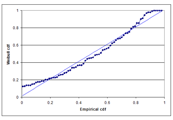
The LED industry used Weibull reliability functions [Philips, ComPlus, CALiPER]. Reference WP12 says, “Philips Lumileds used the Weibull distribution function, a universally-respected statistical technique, to predict the useful lifetimes of power LEDs based on experimental data.” Universal respect is nice, but there is no physical or theoretical justification for the Weibull reliability function. Figure 1 is a P-P plot that shows the Weibull distribution doesn’t fit the DR-03 data set 1, page 5, L70 extrapolations. (A P-P plot is a graph of the empirical (step function) vs. the assumed cumulative distribution function (straight line). Empirical distribution functions put equal probability at each observation.) If the Weibull distribution were a good fit, then the graph would have fit a straight line better. Philips later quit using the Weibull distribution [Philips WP-15].

Philips-Lumileds DR-03 provides sufficient data to estimate L70 reliability, and the data support the inverse-Gaussian L70 model. The partial correlation coefficient between LED test measurements averages ~0.3. After removal of the age factor, the Durbin-Watson statistic [https://en.wikipedia.org/wiki/Durbin%E2%80%93Watson_statistic] for each LED’s lumen measurements indicated little serial correlation, so LED tests might be statistically independent and the deterioration might occur in independent increments, conditions for Brownian motion.

Extrapolating 6000 hour LM-80 LED tests “exponentially” to 60,000 hours [RD-07] and 100,000s of L70 hours is overfitting (162 estimated parameters). The extrapolations don’t represent the variation (Figure 2). Deterioration appears to begin after a few thousand hours. Cree also reports that “lumen maintenance” after 5000 hours differs from earlier. Some alpha and B parameter estimates were inadmissible, resulting in negative L70 ages. The extrapolation parameters should have been computed from the 4000-6000 hour data. 

Alternatives

The 4000 to 6000 hour lumen ratio measurements from DR-03 data sets 1 and 4 pages 5 and 23 appear to have a normal (Gaussian) distributions (figure 3). This implies that L70 has the inverse Gaussian distribution. 

Normal distributions of lumen maintenance ratios could result from geometric Brownian motion with drift [http://en.wikipedia.org/wiki/Black_scholes]. The (natural logarithm of the) lumen maintenance ratio differential equation model lnL(t) is dlnL(t) = mu*lnL(t)dt+sigma*lnL(t)dW(t). This model represents all 80 tested LEDs with two parameters: mu and sigma and normally distributed lumen measurements.

The solution to that differential equation is L(t) = exp[(mu – sigma^2/2)t+ sigma*W(t)] by Ito’s lemma [http://en.wikipedia.org/wiki/Ito%27s_lemma]. (I asked my Probability Theory teacher, Aram Thomasian, “What is Ito’s lemma good for?” He didn’t know either, otherwise we might have become rich from options trading.) Figure 4 shows parameter estimates from DR-03 page 5 data. The estimates of mu and sigma were made from the lumens maintenance ratios ln[L(t+dt)/L(t)], for all t £ 6000 hours. Correction for unequal age intervals took place in the computations. Drift coefficients are slightly negative, and the diffusion coefficient sigma is ~0.0001, after initial observations. 

Figure 5 shows a simulated set of lumen measurements from geometric Brownian motion and the parameters in Figure 4. Figure 5 resembles figure 2 lumens measurements, so geometric Brownian motion could extrapolate the 6000-hour lumen measurements to L70. 

So compute L70 MTTF and reliability from the geometric Brownian motion parameters. This requires a transformation to positive drift. If lnL(t) = v*t+ sigma*W(t), then 1-lnX = min{0<t|lnL(t) = lnX} has the inverse-Gaussian distribution with parameters ln[X/v] and ln[X^2/ sigma^2], where X is a percent of original lumens such as L70 and mu = (v-sigma^2/2). The first parameter is the mean. To keep the parameter n positive, change the sign of mu to represent positive drift so that 1-lnX has the inverse-Gaussian distribution.

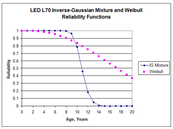
To extrapolate L70, extend each LED’s 6000-hour lumen measurement as geometric Brownian motion [Smith and Lánský]. This yields 80 L70 random variables with 80 independent, equally probable inverse-Gaussian distributions, so the sample distribution of L70 is a mixture of inverse-Gaussian distributions. Figure 6 shows this mixture reliability function. Its MTTF is 95,413  hours, median is 95,574 hours, lower 90% confidence limit on MTTF (B10 L70) is 93,128 hours, and the lower 10^th percentile looks like 10 years. The standard deviation of the mixture is 10,201 hours. The Weibull reliability function in Figure 6 is from the positive L70 extrapolations in reference DR-03 page 5.

Conclusions and Recommendations

Philips Lumileds extrapolations of L70 ages and its confidence limit on MTTF strain credibility. The Weibull reliability function doesn’t fit well. Extrapolation, with different parameters for each tested LED, is overfitting. The wrong range of data appears to have been used for exponential extrapolations, which resulted in some inadmissible, negative L70 age estimates. 

Observed lumen ratio measurements appear to be normally distributed after ~1000 operating hours. This means that geometric Brownian motion could represent drift and variability of lumen maintenance trajectories, after initial deterioration and recovery (2000 and 3000 hours). Geometric Brownian motion of the logarithm of lumens represents measurement drift and variability, parsimoniously, with two parameters. I recommend extrapolating 6000-hour lumens ratios using geometric Brownian motion estimated from 4000 hours on. 

The inverse-Gaussian L70 and other reliability parameters can be computed from the geometric Brownian motion parameters and the desired percentage 70% or other. If you would like the workbooks that produced the figures, let me know.

References

ANSI IES LM-80-21, “Approved Method: Measuring Maintenance of Light Output Characteristics of Solid-State Light Sources,” 2021

ANSI-IES TM21-21, “Technical Memorandum: Projecting Long-Term Luminous, Photon, and Radiant Flux Maintenance of LED Light Sources,“ 2021 

Gouri K. Bhattacharyya and Arthur Fries “Inverse Gaussian Regression and Accelerated Life Tests,” 1982

CALiPER, “Commercially Available LED Product Evaluation and Reporting Program,” PNNL, http://www.netl.doe.gov/ssl/comm_testing.htm

Moon-Hwan Chang, Diganta Das, P.V. Varde, and Michael Pecht “Light Emitting Diodes Reliability Review,” Microelectronics Reliability, Volume 52, Issue 5, pp. 762-782, May 2012

Complus Systems, Ltd. “Understanding Power LED Lifetime,” 

Cree, “XLamp Long-Term Lumens Maintenance,” Cree, Inc., 2009

K. A. Doksum, “Degradation rate models for failure time and survival data,”

CWI Quart, vol. 4, pp. 195–203, 1991

Jiajie Fan, Kam Chuen Yung, and Michael G. Pecht “Lifetime Estimation of High-Power White LED Using Degradation-Data-Driven Method,” IEEE Transactions on Device and Materials Reliability, volume12, pp. 470-477, 2012

George, L. L., “LED Reliability Analysis,” ASQ Reliability Review, Vol. 30, No. 4, pp. 4-11, Dec. 2010

Mark Hodapp “IESNA LM‐80 and TM‐21,” Street Lighting Consortium, Tampa, FL, 2011

Philips, “DR-03: LM-80 Test Report,” http://www.philipslumileds.com/pdfs/DR03.pdf, 2004

Philips, “RD-07: Luxeon Rebel Reliability Data,” http://www.philipslumileds.com/pdfs/DR06.pdf, 2007

Philips, “WP12: Understanding Power LED Lifetime Analysis,” http://www.philipslumileds.com/pdfs/WP12.pdf, undated, also https://www.climateaction.org/images/uploads/documents/Philips_Understanding-Power-LED-Lifetime-Analysis.pdf

Philips, “WP15: Evaluating the Lifetime Behavior of LED Systems,” White Paper 20161201, 2016

Stephen E. Shreve “Did Faulty Financial Models Cause the Financial Fiasco?” Analytics Magazine, Spring 2009

Charles E. Smith and Petr Lánský, “A Reliability Application of a Mixture of Inverse-Gaussian Distributions,” Applied Stochastic Models in Business and Industry, Vol. 10, No. 1, pp. 61-69, 1999

Xiao Wang and Dihua Xu “An Inverse Gaussian Process Model for Degradation Data,” Technometrics, volume 52, pp. 188-197, 2010

Mark White and Joseph B. Bernstein, “Microelectronics Reliability: Physics-of-Failure Based Modeling and Lifetime Evaluation,” NASA-JPL Publication 08-5, 2/08