
The connection between the specifications or drawings or design requirements and the manufacturing process is the capability of the process to consistently create items within spec.
A ratio of the specification over the spread of measured items provides a means to describe the process capability.
The ratios rely on the standard deviation or spread of the produced items. The index is meaningful only if the process is stable. Thus beyond making sure the measurements have minimal measurement error, check the stability using the appropriate control chart.
In this article we are assuming the measurements are normally distributed, yet knowing that is not always the case, you can calculate capability indices using the actual distribution.
The indices will have similar interpretations yet take care when applying these concepts using other than normal distribution data.
Understanding the process capability is useful when:
- Evaluating new vendors, equipment, or processes
- Reviewing design tolerances
- Estimating process yield
- Conducting process audits
- Measuring effect of process changes
The study results in the calculation of one or more process capability indices. Start the study by identifying the measurement and tolerance to evaluate. This may be critical to the quality element of a part or a key indicator of process variation.
Verify the process is stable (often done using control charts described above.) If not stable, take corrective action steps to improve the process by removing special causes of variation. Once stable, then collect data in order to estimate the process standard deviation.
Calculate the desired indices.
Possible Actions
Control charts provide ongoing monitoring of the stability of a process. The capability indices provide a comparison of process variation to the desired tolerance. There are a few possible actions to recommend based on the capability study results.
When the process is capable.
- Continue to monitor. When the process is able to produce items well within the tolerance range you may continue to monitor the process for special causes or reduce or eliminate monitoring depending on risk and monitoring cost.
- Widen the tolerance. If possible, open up the specifications. Of course, this may impact the design and performance. When possible, this option is often less expensive than the next three options.
- Reduce variability. When the spread of the data is large relative to the tolerance range and the data is reasonable centered, then the first step is to reduce the item to item variability. Inspection or sorting is not a good option here, rather improve the process to reduce the sources of the variability. This may involve changing the technology within the process, automating steps and/or improving training and feedback for manual processes.
- Center the process. If if the center of the measurements is not aligned with the target of the specification, adjust the process to shift the center of the produced items. This is often simpler to accomplish than reducing variation, yet may have little effect if the variation is large. Best done when the spread of the data would theoretically create a capable process if only centered.
- Accept the losses. This is a business decision. When the options above are either not technically feasible or cost prohibitive, then the option to accept the items out of tolerance and the resulting impact on quality, reliability or performance is the only option.
Knowing how to interpret the results and which actions will lead to improved designs and processes, allows the team to create robust and durable products.
Estimating Process Spread
If using control charts then we can use the range of the samples from an X-bar & R chart, for example, to estimate the individual item standard deviation.
Also, if we have the individual readings, we can directly calculate the standard deviation.
Cp Process Capability Index
Once we have an estimate of the standard deviation of the measurement of interest and the respective tolerance range, we can calculate the process capability index, Cp.
$$ \large\displaystyle Cp=\frac{\left( USL-LSL \right)}{6\sigma }$$
USL is the upper specification or tolerance limit
LSL is the lower specification or tolerance limit
σ is the standard deviation of the measurements from a stable process
A Cp of 1.0 means the process and tolerance spreads are equal.
The data is from an example dataset and is 125 diameter readings. I adjusted the tolerance range to be centered on the average of the data and plus/minus 3 σ. The plot is created using R and the qcc package.
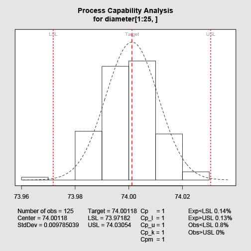
The plus/minus 3 σ line up with the specification limits. Any variation of the center or spread of the process will increase the number of items falling out of the tolerance range. Processes do vary.
Also, not the Cp formula does not account for the location of the measurements. It just compares the spreads, not their alignment.
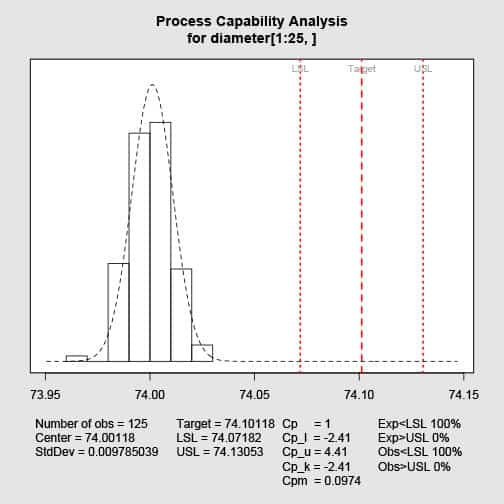
The Cp is still one, yet none of the items are within spec.
For any Cp calculation, check the plot of the histogram versus the specifications.
In general:
Cp > 1.33 the process is capable
Cp = 1.00 to 1.33 the process is marginally capable
Cp < 1.00 the process is incapable
This set of definitions is arbitrary. When the process creates item measurements with a normal distribution, and the Cp = 1, we will expect a defect rate of 2,700 ppm*. Meaning for a production of one million items, 2,700 will be outside the specifications if and only if the process remains stable and centered. *ppm is part per million (10^6).
For a Cp = 1.33, we expect a defect rate of 63 ppm. For each project compare the defect rates to the goal defect rates for the specific part or dimension. In general, the more complex and higher part count the system, the higher the Cp values desired with every process.
The following table provides the Cp and corresponding ppm values assuming a perfect normal distribution that is stable and centered.
| Cp | ppm |
|---|---|
| 0.33 | 317,311 |
| 0.67 | 45,500 |
| 1.00 | 2,700 |
| 1.10 | 967 |
| 1.20 | 318 |
| 1.30 | 96 |
| 1.33 | 63 |
| 1.40 | 27 |
| 1.50 | 6.8 |
| 1.60 | 1.6 |
| 1.67 | 0.57 |
| 1.80 | 0.0067 |
| 2.00 | 0.002 |
Higher Cp values indicate the process is able to produce parts that could fit within the tolerance range and accommodate the naturally occurring shifts in the mean and standard deviation values over time while remaining in spec.
The Cpk index
Cpk Considers the location of the average reading in relationship to the tolerance limits. Like the Cp is is a ration of specification range over process spread, yet incorporates the centering of the data relative to the tolerance.
The Cpk calculation is
$$ \large\displaystyle Cpk=\min \left\{ \frac{\left( USL-\bar{X} \right)}{3\sigma },\frac{\left( \bar{X}-LSL \right)}{3\sigma } \right\}$$
Where X-bar is the mean of the measurements.
The Cp and Cpk are equal when the data is centered (and a normal distribution). And, not equal when the data is offset from the center.
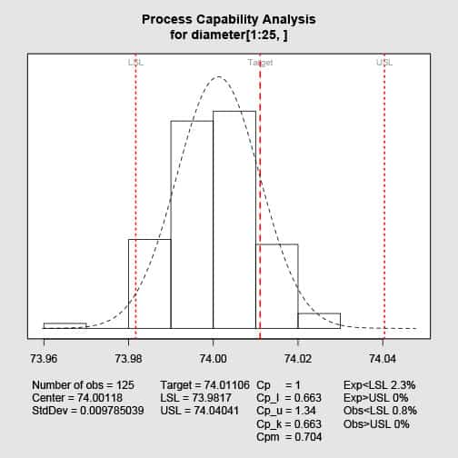
Using the same data as in the plots in the Cp discussion and shifting the specification up just one standard deviation (effectively moving the data lower or closer to the lower spec) we find the Cpk values is 0.663.
The same guidelines to interpret the Cpk values apply as with the Cp values. In this case, with Cpk = 0.663 we would conclude the process in not capable. The plot and value suggest that centering the process may create a marginally capable process. The team should consider opening the specifications and reducing the variability to further improve the process capability.
The Cpm index
One assumption of the Cp and Cpk indices is the optimal value is centered between the tolerance limits. This is not always the case, thus consider using the index Cpm. This index also is a ration of tolerance range over process spread and it adjusts for the location of the target relative to the center of the data.
Calculate Cpm
$$ \large\displaystyle Cpm=\frac{\left( USL-LSL \right)}{6\sqrt{{{\left( \bar{X}-T \right)}^{2}}+{{\sigma }^{2}}}}$$
Where T is the target value.
Using the same data and limits as in the Cpk example, and adding a target value of 73.998 we find
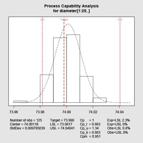
With a Cpm value of 0.951, which is still not capable yet would estimate more of the items would be near the target than the Cpk would estimate.
Related:
Pre-Control Charts (article)
Variable Selection for Control Charting (article)
Chance of Catching a Shift in a Control Chart (article)

very nice and simplified presentation . thanks.