Priorities, priorities…

This is the sixth edition of the R for Engineering newsletter, and today we look at the ultimate prioritization tool – Pareto charts!

Pareto charts are a core tool for anyone who makes decisions, whether it is selecting a project or problem to solve, combing through last year’s spend or deciding on what equipment to purchase this year. The list goes on; bottom line is that Pareto charts simply allow you to focus on what’s important and cut through what may be interesting but unimportant.

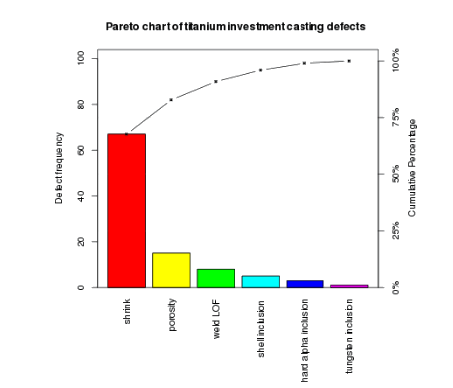
The good news is that Pareto charts are fairly easy to interpret as long as they are consructed in a way that facilitates understanding. I am honestly not a fan of traditional Pareto charts where the bars for each categorical variable are plotted on the X axis, which ends up making it hard to read the labels. To add insult to injury, traditional Pareto charts feature a second visual, which is the cumulative percentage of the categories plotted on the right side of the Y axis. This guarantees a cacophonic experience when listening to what the chart is trying to tell you…

Below is an example of what I mean – it is literally from the Wikipedia page for Pareto charts.

Instead, my preferred approach is flipping the axes and simply omitting the cumulative line as it adds no additional information that the bars don’t already provide. Flipping the axes also allows reading the labels without having to turn your head sideways.

All of this can certainly be done in R using the ggplot2 package, and although it’s not super hard to do, I had decided to create a custom function—actually, two custom functions—to make creating Pareto charts a seamless experience for myself and others.

Let’s walk through how to do it. To demonstrate how to create and customize the chart, I am going to be using a dataset that has all automobile recalls issued by National Highway Traffic Safety Administration from 1966 to January 2023,both the vehicle and the subsystem level. That’s a lot of data, 50,000+ individual entries.

# WEEK 006: PRIORITIES, PRIORITIES - PARETO CHARTS

# 0. LIBRARIES

# install.packages("devtools")
devtools::install_github("gaborszabo11/sherlock")

 
library(tidyverse)
library(sherlock)


# 1. LOAD FILE ----
auto_recalls <- load_file("https://raw.githubusercontent.com/gaboraszabo/datasets-for-sherlock/main/auto_recalls_1966_2023.csv", ".csv")

Now that we’ve loaded the packages and read in the data, let’s call the function draw_pareto_chart().

# 2.1 PARETO CHART FOR NUMBER OF RECALLS BY TYPE OF COMPONENT, 1966-2023 ----
auto_recalls %>%
  draw_pareto_chart(cat_var = Component, summarize = TRUE)

The above Pareto chart simply shows the number of recalls by component or subsystem from 1966 to 2023. Interesting; the heaviest hitter seems to be equipment, which is rather generic. Let’s try and dig a little deeper as well as customize the chart.

# 2.2 PARETO CHART FORMATTED ----
auto_recalls %>%
  draw_pareto_chart(cat_var   = Component,
                    summarize = TRUE,
                    highlight_first_n_items = 1,
                    lump_last_n_items       = 20,
                    lumped_cat_name         = "Other Components", 
                    title_label             = "NHTSA Automobile Recalls, 1966-2023")

As far as customization, we could highlight the first n items and/or lump the last n items into one bucket. We could also give the chart a better title. OK, let’s do that.

The chart now looks much more visually appealing but we may still want to better understand what equipment means and if it really has been the most important of all type of recalls throughout the years.

Let’s use a function that allows drilling down another layer, and that is draw_pareto_grouped(). This simply enables grouping by an additional variable, which will be Recall Type, and it could be either Vehicle (vehicle-level) or Equipment (sub-system level). Let’s see what this look like:

# 2.3 GROUPED PARETO FOR NUMBER OF RECALLS BY TYPE OF COMPONENT GROUPED BY TYPE OF RECALL, 1966-2023 ----
auto_recalls %>%
  draw_pareto_chart_grouped(cat_var      = Component,
                            grouping_var = `Recall Type`,
                            summarize    = TRUE,
                            highlight_first_n_items = 1, 
                            title_label  = "NHTSA Automobile Recalls, 1966-2023")

Still not much insight as the first item on both displays is equipment… At this point, if you haven’t already, you may want to consider thinking about what could make a recall more important than other recalls. One thing one can think of is the number of vehicles affected. Thankfully, this data has been provided for each of the recalls, and with a little bit of calculation, we are able to sum up the number of vehicles affected for each component and recall type. Here we go:

# 2.4.1 FIXED X AXIS FOR COMPARISON ----
auto_recalls %>%
  group_by(`Recall Type`, Component) %>%
  summarize(Sum_Potentially_Affected = sum(`Potentially Affected`)) %>%
  drop_na() %>%
  draw_pareto_chart_grouped(cat_var = Component,
                            grouping_var = `Recall Type`,
                            summarize = FALSE,
                            continuous_var = Sum_Potentially_Affected,
                            x_axis_span = "fixed",
                            highlight_first_n_items = 1, 
                            title_label    = "NHTSA Automobile Recalls by Component by Recall Type, 1966-2023", 
                            analysis_desc_label = "Number of vehicles potentially affected")

This looks very different, right? It looks like at the vehicle level, the one component or sub-system that has (potentially) affected the most vehicles is the air bag with well over 100,000,000 vehicles potentially affected over the years. At the equipment (or component) level, we are looking at tires as the highest-ranking items having potentially affected over 30,000,000 vehicles. Setting the x_axis_span argument to “fixed” also allowed us to compare the two categories side by side, relative to one another (small multiples in action!), which tells us that far more vehicles have been affected at the vehicle-level than at the component level.

Hope you enjoyed this week’s edition.

Resources:

• Code – GitHub repo
• R for Data Science reference book
• sherlock package
• draw_pareto_chart() function documentation