
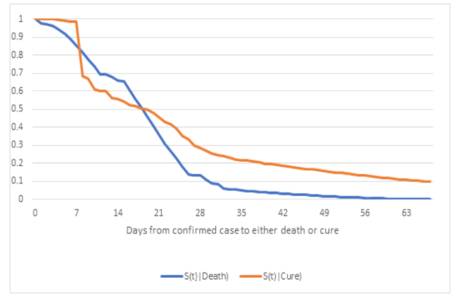
“It is the policy of my Administration to respond to the coronavirus disease 2019 (COVID-19) pandemic through effective approaches guided by the best available science and data” [Biden Executive order, 2021]. That epidemic inspired the simultaneous nonparametric estimation of survival functions from case to recovery and case to death, without lifetime data (figure 1)!
Why not do the same for multiple-failure-mode data? This article shows nonparametric, multiple-failure-mode, maximum likelihood reliability estimation in a spreadsheet. Data are system first-failure times and the corresponding failure modes that caused the first system failures (table 1). However those data are dependent. I will explain the likelihood function, lnL, and how to find the maximum likelihood reliability estimates for all failure modes simultaneously.
Some articles and statistical software use Kaplan-Meier estimators for each failure mode [Dignam et al., ReliaSoft-ReliaWiki, Minitab, Others?]. Unfortunately, the Kaplan-Meier estimator is for independent, identically distributed, perhaps censored data [Mailman School of Public Health, Prentice et al., Yizeng He et al., Thernau et al. 2024, Lin et al.]. Using Kaplan-Meier results in reliability estimates that are biased low.
Simultaneous estimates could be produced by constrained least squares; e.g., COVID-19 “survival” function estimation in two modes: recovery and death, from periodic case, recovery, and death counts (figure 1) [George 2021]. Why not maximize the multiple-mode likelihood function constrained by the percentages of failures in each mode [Prentice et al., George 2025]? Table 1 shows some multiple-mode, first-failure time data for example.
Table 1. Multiple-Mode, first-failure-time data (first three columns) [Rao, Meeker et al.] and likelihoods
| Kilometers | Fail Mode | Censored? | L=Likelihood | lnL |
| 6700 | Mode1 | Failed | 0.01681 | -4.0857 |
| 6950 | Censored | Censored | 0.98319 | -0.017 |
| 7820 | Censored | Censored | 0.98319 | -0.017 |
| 8790 | Censored | Censored | 0.98319 | -0.017 |
| 9120 | Mode2 | Failed | 0.01836 | -3.9978 |
| 9660 | Censored | Censored | 0.96483 | -0.0358 |
| 9820 | Censored | Censored | 0.96483 | -0.0358 |
| 11310 | Censored | Censored | 0.96483 | -0.0358 |
| 11690 | Censored | Censored | 0.96483 | -0.0358 |
| 11850 | Censored | Censored | 0.96483 | -0.0358 |
| 11880 | Censored | Censored | 0.96483 | -0.0358 |
| 12140 | Censored | Censored | 0.96483 | -0.0358 |
| 12200 | Mode1 | Failed | 0.02032 | -3.8961 |
| 12870 | Censored | Censored | 0.94451 | -0.0571 |
| 13150 | Mode2 | Failed | 0.02168 | -3.8312 |
| 13330 | Censored | Censored | 0.92283 | -0.0803 |
| 13470 | Censored | Censored | 0.92283 | -0.0803 |
| 14040 | Censored | Censored | 0.92283 | -0.0803 |
| 14300 | Mode1 | Failed | 0.02225 | -3.8056 |
| 17520 | Mode1 | Failed | 0.02225 | -3.8056 |
| 17540 | Censored | Censored | 0.87833 | -0.1297 |
| 17890 | Censored | Censored | 0.87833 | -0.1297 |
| 18450 | Censored | Censored | 0.87833 | -0.1297 |
| 18960 | Censored | Censored | 0.87833 | -0.1297 |
| 18980 | Censored | Censored | 0.87833 | -0.1297 |
| 19410 | Censored | Censored | 0.87833 | -0.1297 |
| 20100 | Mode2 | Failed | 0.02783 | -3.5817 |
| 20100 | Censored | Censored | 0.85051 | -0.1619 |
| 20150 | Censored | Censored | 0.85051 | -0.1619 |
| 20320 | Censored | Censored | 0.85051 | -0.1619 |
| 20900 | Mode2 | Failed | 0.03086 | -3.4783 |
| 22700 | Mode1 | Failed | 0.02878 | -3.5482 |
| 23490 | Censored | Censored | 0.79087 | -0.2346 |
| 26510 | Mode1 | Failed | 0.02987 | -3.5107 |
| 27410 | Censored | Censored | 0.761 | -0.2731 |
| 27490 | Mode1 | Failed | 0.03108 | -3.4712 |
| 27890 | Censored | Censored | 0.72992 | -0.3148 |
| lnL-> | -44.013 |
Spreadsheet Implementation
You could copy this article’s tables into your own spreadsheet, or you could ask for my spreadsheet with cell formulas. Some work is required to reproduce the formulas that generate the numbers in tables 1-4. I hope the following explanation explains how to do it.
The dependence among failure modes is represented by the proportions of failures in the 38 independent random samples in which each failure mode is the first failure, table 2. Kaplan-Meier estimates by failure mode do not yield these proportions. Some people have tried to use the failure mode as a factor in Kaplan-Meier, proportional hazards, reliability estimates [Agrawal et al.], using statistical software [e.g., Thernau “Survival” R-package].
Table 2. Failure proportions and counts out of 38 in table 1: 27 were both censored
| Mode | Proportion |
| Mode1 | 0.18421 |
| Mode2 | 0.10526 |
| Failure Counts | |
| Mode1 | 7 |
| Mode2 | 4 |
| Total | 38 |
For each observation time t, the likelihoods in table 1 consists of terms such as p(t;mode)*(1-F(t;other mode) if failure at age t or (1-F(t;mode)*(1-F(t;other mode). The p(t;.) is the discrete probability of failure at age t, and F(t;.) is the discrete cumulative distribution function of time or kilometers to failure. Reliability is (1-F(t;mode)). Likelihood L is the product of all of the terms. The product could cause underflow, so maximize the sum of the logarithms of the likelihoods. For more detailed explanation about inappropriate and appropriate likelihood function(s) for multiple mode failure data, please refer to https://fred-schenkelberg-project.prev01.rmkr.net/statistical-software-problem/.
Table 3 contains estimates of p(t;mode), and table 4 contains the corresponding reliability estimates R(t;mode)=1-F(t;mode) computed from table 3. Tables 3 and 4 are used in table 1 to construct the likelihoods row by row, manually, using either p(t;mode)*(1-F(t;other mode) if failure at age t or 1-F(t;mode1)*(1-F(t; mode2) depending on censoring. Nested IF(IF()) statements could do the same, less clearly. Table 3 could be copied anywhere convenient in a spreadsheet. Table 4 should be copied so its rows line up with table 1 for convenience.
Table 3. Discrete probabilities of failures at ages (km) t: p(t;mode). He “KM p-h ” p(t;mode) estimates are derived from the Kaplan-Meier proportional hazards (modes) estimates
| Km | p(t;mode1) | p(t;mode2) | KM p-h 1 | KM p-h 2 |
| 6700 | 0.01681 | 0 | 0.0263 | |
| 9120 | 0 | 0.01867 | 0.0286 | |
| 12200 | 0.02071 | 0 | 0.0364 | |
| 13150 | 0 | 0.02253 | 0.0379 | |
| 14300 | 0.0232 | 0 | 0.0435 | |
| 17520 | 0.0232 | 0 | 0.0435 | |
| 20100 | 0 | 0.03038 | 0.0653 | |
| 20900 | 0 | 0.03369 | 0.0898 | |
| 22700 | 0.03216 | 0 | 0.0899 | |
| 26510 | 0.03339 | 0 | 0.1077 | |
| 27490 | 0.03474 | 0 | 0.1437 | |
| Sums | 0.18421 | 0.10526 | 0.491 | 0.2216 |
| Proportions | 0.18421 | 0.10526 |
Table 4 is built from table 3 p(t;mode) as R(t;mode)=1-∑p(s;mode), s=1,2,…,t, at failure times t in each mode. F(t;mode) is constant in between modal failure times. KM1 and KM2 are the Kaplan-Meier reliability estimates for each failure mode. Notice that reliability R(28100 km;mode1)=0.81579=1-0.18421 and R(28100 km;mode2)=0.89474=1-0.10526 agrees with the failure proportions in table 2. The Kaplan-Meier estimates KM1 and KM2, at 28100 km disagree.
Table 4. R(t;mode)=1-F(t;mode) estimates, from the sums, F(t;mode)=∑p(s;mode) s=1,2,…,t.
| Km | R(t;Mode1) | R(t;Mode2) | KM1 | KM2 |
| 0 | 1 | 1 | 1 | 1 |
| 6700 | 0.98319 | 1 | 0.97368 | 1 |
| 6950 | 0.98319 | 1 | 0.97368 | 1 |
| 7820 | 0.98319 | 1 | 0.97368 | 1 |
| 8790 | 0.98319 | 1 | 0.97368 | 1 |
| 9120 | 0.98319 | 0.98133 | 0.97368 | 0.97059 |
| 9660 | 0.98319 | 0.98133 | 0.97368 | 0.97059 |
| 9820 | 0.98319 | 0.98133 | 0.97368 | 0.97059 |
| 11310 | 0.98319 | 0.98133 | 0.97368 | 0.97059 |
| 11690 | 0.98319 | 0.98133 | 0.97368 | 0.97059 |
| 11850 | 0.98319 | 0.98133 | 0.97368 | 0.97059 |
| 11880 | 0.98319 | 0.98133 | 0.97368 | 0.97059 |
| 12140 | 0.98319 | 0.98133 | 0.97368 | 0.97059 |
| 12200 | 0.96248 | 0.98133 | 0.93623 | 0.97059 |
| 12870 | 0.96248 | 0.98133 | 0.93623 | 0.97059 |
| 13150 | 0.96248 | 0.9588 | 0.93623 | 0.93015 |
| 13330 | 0.96248 | 0.9588 | 0.93623 | 0.93015 |
| 13470 | 0.96248 | 0.9588 | 0.93623 | 0.93015 |
| 14040 | 0.96248 | 0.9588 | 0.93623 | 0.93015 |
| 14300 | 0.93928 | 0.9588 | 0.88942 | 0.93015 |
| 17520 | 0.91608 | 0.9588 | 0.84261 | 0.93015 |
| 17540 | 0.91608 | 0.9588 | 0.84261 | 0.93015 |
| 17890 | 0.91608 | 0.9588 | 0.84261 | 0.93015 |
| 18450 | 0.91608 | 0.9588 | 0.84261 | 0.93015 |
| 18960 | 0.91608 | 0.9588 | 0.84261 | 0.93015 |
| 18980 | 0.91608 | 0.9588 | 0.84261 | 0.93015 |
| 19410 | 0.91608 | 0.9588 | 0.84261 | 0.93015 |
| 20100 | 0.91608 | 0.92842 | 0.84261 | 0.85263 |
| 20100 | 0.91608 | 0.92842 | 0.84261 | 0.85263 |
| 20150 | 0.91608 | 0.92842 | 0.84261 | 0.85263 |
| 20320 | 0.91608 | 0.92842 | 0.84261 | 0.85263 |
| 20900 | 0.91608 | 0.89474 | 0.84261 | 0.74606 |
| 22700 | 0.88391 | 0.89474 | 0.72224 | 0.74606 |
| 23490 | 0.88391 | 0.89474 | 0.72224 | 0.74606 |
| 26510 | 0.85053 | 0.89474 | 0.57779 | 0.74606 |
| 27410 | 0.85053 | 0.89474 | 0.57779 | 0.74606 |
| 27490 | 0.81579 | 0.89474 | 0.38519 | 0.74606 |
| 27890 | 0.81579 | 0.89474 | 0.38519 | 0.74606 |
| 28100 | 0.81579 | 0.89474 | 0.38519 | 0.74606 |
Figure 2 shows the bias in the Kaplan-Meier reliability proportional-hazards estimates (KMPH) compared with the maximum likelihood estimates. The lines are the maximum likelihood reliability estimates, and the dots are the Kaplan-Meier proportional hazards estimates.

Figure 3 shows the nonparametric maximum likelihood discrete failure rate function estimates, at times (kilometers) of failures by failure mode. The proportional hazards assumptions seems reasonable, even if the resulting reliability estimates In Figure 1 are biased. That bias is because independent, Kaplan-Meier, proportional hazards estimates do not account for the dependence in proportions of modal failures.

Maximum Likelihood estimation
Use Excel Solver to maximize lnL (below table 1) as a function of the p(t;mode) values in table 3. Set a constraint that the sums of failure mode probabilities,∑p(s;mode), equal the proportions in table 2. I tried doing maximization on table 4 directly, but Excel complained about too many variables.
Recommendations
Don’t use the Kaplan-Meier reliability function estimates for multiple-mode first-failure times, because they don’t account for observed proportional dependence among the failure modes. They are biased low because, for the older failure times, each Kaplan-Meier reliability estimate are multiplied by (1-1/survivors)->0 as the number of survivors decreases.
Doubt statistical software the allows specifying parametric distributions for each failure mode. They may use parameter estimates in each failure mode separately without accounting for dependence. I failed to make the maximum likelihood estimation work for Weibull reliability functions on another data set with the proportionality constraint.
One paper describes using a bivariate Weibull distribution estimate, analogous to the Marshall-Olkin bivariate exponential distribution. That accounts for simultaneous failures, if any [Agrawal et al.].
Why not do multiple-mode reliability estimation, without lifetime data? Joe Biden says so [Executive Order]! Even with multiple-mode data? Generally Accepted Accounting Principles requires statistically sufficient data, and it’s population data! It is reasonable to count failures by failure mode; e.g., product sales, BoMs, and simultaneous spare parts’ sales or demands; Corona Virus case, recovery, and death counts [George 2025].
References
Aakash Agrawal, Debanjan Mitra, and Ayon Ganguly, “A Model for Censored Reliability Data with Two Dependent Failure Modes and Prediction of Future Failures,” arXiv:2206.12892v1 [stat.ME], 26 Jun 2022
Joseph Biden, “Executive Order on Ensuring a Data-Driven Response to COVID-19 and Future High-Consequence Public Health Threats,” Jan. 21, 2021
James J Dignam, Qiang Zhang, Maria N, Kocherginsky, “The Use and Interpretation of Competing Risks Regression Models,” Clin Cancer Res.;18(8):2301–2308. doi: 10.1158/1078-0432.CCR-11-2097, Jan. 2012
L. L. George, “COVID-19 Survival Analysis,” https://sites.google.com/site/fieldreliability/corona-virus-survival-analysis/ Jan. 2021
L. L. George, ”Statistical Software Problem,” https://fred-schenkelberg-project.prev01.rmkr.net/statistical-software-problem/#more-582018/, Jan. 2025
Yizeng He, Kwang Woo Ahn , Ruta Brazauskas, “A Review of Competing Risks Data Analysis,” https://www.mcw.edu/-/media/MCW/Departments/Biostatistics/TR070.pdf/
Guixian Lin, Ying So, Gordon Johnston, “Analyzing Survival Data with Competing Risks Using SAS® Software,” SAS Global Forum 2012
Meeker, William Q. and Luis A. Escobar, “Degradation Data, Models, and Data Analysis,” 2003, http://www.public.iastate.edu/~wqmeeker/stat533stuff/psnups/chapter13_psnup.pdf
E. L. Kaplan and P. Meier, ”Nonparametric Estimator From Incomplete Observations,” J. Amer. Statist. Assn., Vol. 53, pp. 457-481, 1958
Mailman School of Public Health, “Competing Risk Analysis,” Columbia U. Irving Medical Center, https://www.publichealth.columbia.edu/research/population-health-methods/competing-risk-analysis#/
Ross L. Prentice, J. D. Kalbfleisch, A. V. Peterson, N. Flournoy, V. T. Farewell, and N. Breslow, “The Analysis of Failure Time Data in the Presence of Competing Risks,” Biometrics, Vol. 34, pp. 541-554, 1978
Ross L. Prentice and J. D. Kalbfleisch, “Hazard Rate Models with Covariates,” Biometrics, Vol. 34, No. 1, Perspectives in Biometry, pp. 25-39, March 1979
Reliasoft-Reliawiki, “Competing Failure Modes (CFM) Analysis,” https://www.reliawiki.com/index.php/Competing_Failure_Modes_Analysis/, Sept. 2023
Terry Thernau, “Package ‘survival,’” https://github.com/therneau/survival/, Dec. 2024
Terry Therneau, Cynthia Crowson, and Elizabeth Atkinson, “Multi-state models and competing risks,” https://cran.r-project.org/web/packages/survival/vignettes/compete.pdf/, December 17, 2024

This is a link to the Google Sheet that is described in the Multiple-Failure-Mode article;
https://docs.google.com/spreadsheets/d/1iH-u71STujVm-C7S2bp3xmoJBOxLOFC9xfBQn-10ndA/edit?usp=sharing/
You can see the cell formulas in that sheet, but Google won’t do the optimization to find the max. likelihood nonparametric reliability estimates (already shown, for the input data in table 1).
Copying and pasting my email response here.
====================================================
Hello Dr. George,
My apologies for the late reply. I was caught up with some work and couldn’t get the time to look into this.
Thanks for writing the article! I do have some thoughts on it that I wanted to share with you.
Suppose we have only 2 modes of failure – mode 1 and mode 2. I am assuming that you are trying to answer questions of the type: What is the probability of failure from mode 1 by time “t” AND this failure occurs before mode 2? If my assumption is right, then this is the exact definition of the cumulative incidence function, also called the sub-distribution function. Using Kaplan Meir estimator in a competing risk context is different to the cumulative incidence function. The Kaplan Meir estimator for mode 1 failures is calculated by treating mode 2 failures as “censored”. This would give us the probability of a mode 1 failure in a hypothetical world where failures can occur ONLY due to mode 1 and not due to mode 2. Unless mode 2 is eliminated by changing design, we are still interested in a world where modes 1 and 2 are both possible. I agree that we should not use the Kaplan Meir approach in a real-world scenario where both modes are active. But I am a bit confused as to why you seem to equate the Kaplan Meir approach with the cumulative incidence function, since both are different. The cumulative incidence of mode 1 takes into account the rate at which mode 2 failures are occurring. Also, the non-parametric version of the cumulative incidence function can be estimated without making any assumptions of the joint distribution of the failure times of the 2 modes of failures. So, we are not making any assumptions of independence of the time-to-failure of the two modes.
Now, coming back to the original question of interest: What is the probability of failure from mode 1 by time “t” AND this failure occurs before mode 2? I see that you have used a likelihood-based approach and have constrained the maximization to the observed proportions of the two failure modes. I have to admit, I am not familiar with this approach to answering the above question. Doesn’t mean I don’t think it is correct! Just that I am not sure why we would have 2 different answers to the same probabilistic question. Unless you are trying to answer a different question altogether?
Would love to hear your thoughts on this.
Regards,
Shishir.
PS: Do you mind if I post this comment on your article? I think this is a good discussion and others might benefit from it and there is a possibility that others might chip in their 2 cents.
====================================================
Thanks. I was unfamiliar with the cumulative incidence function and was trying to estimate the conditional reliability functions R(t|failure mode 1) and R(t|failure mode 2) and their joint distribution function to test for independence.
I asked Google AI, “What’s wrong with Kaplan-Meier for multi-mode reliability estimation from censored lifetime data?
Google AI replied: “Using a Kaplan-Meier reliability estimator with multiple mode lifetime failure data is problematic because the Kaplan-Meier method is designed to analyze a single failure mode, meaning it cannot accurately capture the different failure mechanisms present in a dataset with multiple modes of failure, potentially leading to misleading results when trying to estimate overall reliability.
Key reasons why Kaplan-Meier is not suitable for multiple mode failure data:
Assumption of a single failure process:
The Kaplan-Meier method assumes that all failures occur due to a single underlying process, while multiple mode failure data implies different failure mechanisms with distinct failure times, violating this assumption.
Inability to differentiate failure modes:
When analyzing multiple failure modes with Kaplan-Meier, you cannot identify which failure mode caused each event, leading to an inaccurate representation of the overall reliability.
Misinterpretation of survival curve:
The Kaplan-Meier curve generated from multiple mode data could be misinterpreted as representing a single failure mode, potentially leading to incorrect conclusions about system reliability.
Alternative approaches for multiple mode failure data:
Competing risks analysis:
This method explicitly accounts for different competing failure modes by estimating the probability of each failure mode occurring, given that another mode has not already occurred.
Failure mode specific analysis:
Analyze each failure mode separately using Kaplan-Meier, but interpret the results carefully considering the potential interactions between different modes.
Parametric models:
If the underlying distributions of each failure mode are known, use parametric models that can incorporate multiple failure mechanisms.”
Hello Dr George, I would also suggest looking into the issue of “non-identifiability” of dependence among failure modes in competing risks (also called “identifiability dilemma”). It basically says that, given what we are able to observe in a competing risks framework (T, j), where “T” is the time to failure and “j” is the failure mode, it is not possible to say anything about the dependence structure between the risks. The observed data could have come from a joint distribution with strong, weak or no dependence at all – we cannot say.
This Google Sheet shows the joint probability density max. likelihood estimates of {p(s|mode 1, p(t|mode 2)} in table 3 of
https://docs.google.com/spreadsheets/d/1iH-u71STujVm-C7S2bp3xmoJBOxLOFC9xfBQn-10ndA/edit?usp=sharing/
It’s for age s and t values up to the oldest failures in either failure mode.