MTBF free Availability

The classic formula for availability is MTBF divided by MTBF plus MTTF. Standard. And pretty much wrong most of the time.

Recently, working for a bottling plant design team, we pursued design options to improve the availability and throughput of the new line. The equipment would remain the same: filler, capper, labeler, etc. So we decided to gather the last six months or so of operating data, which included up and down time. Furthermore, the data included time to failure and time to repair information.

MTBF Using Assumed Exponential Distribution

The plant traced availability using the classic formula, simply the total operating or up time by the total run time. We learned during plant visits that the longer runs tended to get better availability. The data, looking at short runs (1 day) versus long runs (5 days), did show a marked difference in availability. It also revealed the MTBF went up with longer runs. The MTTR remained pretty constant or went up just a little.

Recall we have the ‘time to’ data. A little work with a spreadsheet, and we fit distributions to the data: Weibull, Lognormal, and Exponential fit different equipment results. And we had a wealth of data, permitting excellent data analysis and distribution fit decisions. While each piece of equipment had many failure types, each had one dominant failure mechanism. For the sake of this article, let’s assume the equipment operating time is well described by a Weibull distribution with a beta of less than 1. The lognormal distribution well describes the time to repair data. While this wasn’t universal across all the types of bottles and equipment, it will work for this article.

So why do we commonly use MTBF with the assumption of an underlying exponential distribution? There are many reasons: ignorance, “always done that way,” lack of ‘time to’ data, or in rare cases, the assumption is valid. Let’s remove the ignorance excuse and ‘always….’ and make the case for using an appropriate analysis with appropriate assumptions simultaneously.

Why is using MTBF so bad for availability calculations?

Let’s look at one example: the design of the bottling line. The high-volume bottling process has up to 10 steps, each involving highly complex and expensive equipment. The design team was balancing the line availability and throughput per shift with the cost of the equipment. The other part of the design consideration was the cost of storing finished goods with the change over time between flavors and bottle sizes. The idea was to add just enough redundant equipment to change the line over time, and line availability permitted frequent line changes, significantly reducing finished goods storage costs.

Each flavor and bottle size combination would have a dedicated line in a perfect plant. In reality, the expected run times of the flavor and bottle size combinations ranged from a few hours per month to two weeks a month, with most running for less than a week. Also, consider the equipment costs a few million dollars per unit.

Therefore, we built an availability model of the existing line configuration and the various proposed line configurations. The model would permit the simulation of various expected line management policies to determine the ability to reduce finished goods storage costs. The model would significantly influence the million-dollar decisions in the project.

Back to why we want to look at the underlying and common assumption – MTBF and MTTR often assume the exponential distribution. This distribution does not account for changes in the failure or repair rate. The first hour and any hour of operation after that have precisely the same average failure rate or repair rate.

Fitting the Data That Changes Over Time

Recall the observation and supporting data that suggest neither MTBF nor MTTR are constant. Both seem to depend to some degree on the length of the run. I’m a statistician, and the plant had years’ worth of data on the equipment. Happiness.

First, get the data and determine the best-fitting distribution. This is a simple regression analysis. Here is an example of the difference between assuming the exponential and fitting a distribution.

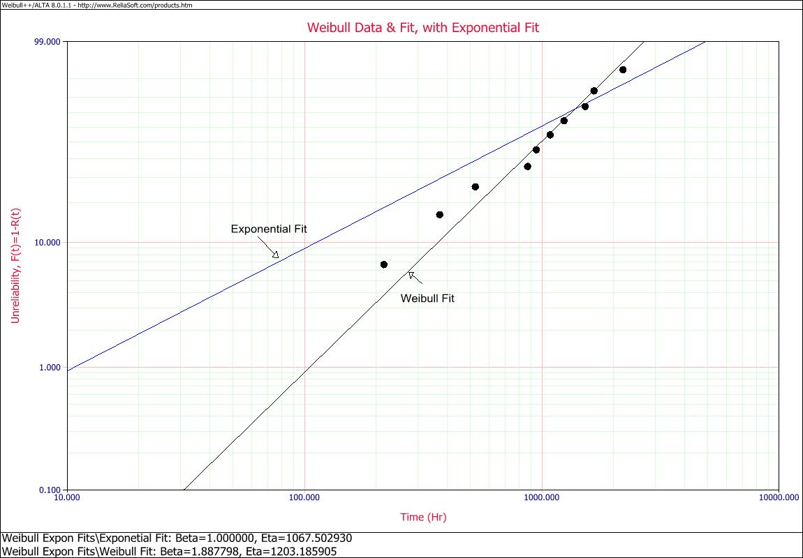
The data was drawn randomly from a Weibull Beta 2 Eta 1000 distribution. The Weibull fit is pretty good, as expected. Forcing the fit to exponential overestimates the failure rates at earlier times, and those earlier times of often of most interest.

Second, determine how to calculate availability given the fitted distributions. This second step had me hitting the books.

The general formula for calculating availability is based on expected values, not MTBF and MTTR based on exponential distributions. ‘Expected Values’ If you are like most engineers, you may only have a vague recollection of this statistical term. Most associated this phrase with the mean or average value, which is mostly true. The availability formula changes from

$$ \displaystyle A=\frac{\text{MTBF}}{\text{MTBF}+\text{MTTR}}$$

to this

$$ \displaystyle A=\frac{{{E}_{failures}}}{{{E}_{failures}}+{{E}_{repairs}}}$$

If you are familiar with the Weibull distribution, you recall if the beta is equal to 1, the characteristic life is the theta. The same as for an exponential distribution. When the beta is not equal to one, the characteristic life is not equal to theta. The mean is another way to say the expected value.

For the exponential distribution the expected value calculation is very commonly used to calculate MTBF.

$$ \displaystyle {{E}_{Expontential}}=\frac{1}{\lambda }$$

Whereas, for the Weibull distribution the formula is

$$ \displaystyle {{E}_{Weibull}}=\lambda \Gamma \left( 1+\frac{1}{\beta } \right)$$

and, for the Lognormal distribution the formula is

$$ \displaystyle {{E}_{Lognormal}}={{e}^{\mu +\frac{1}{2}{{\sigma }^{2}}}}$$

Therefore, we calculate the expected values and determine the availability. Note: the expected value of a distribution is not always the same as the characteristic life. For example, the expected value of a Weibull distribution is not the characteristic life or eta; it, in part, depends on the beta parameter, thus often different than the characteristic life. We get a better estimate of availability, all while using the data described adequately with the appropriate distribution. Easy.

Note: reviewing this analysis approach with other statisticians, they recommended, given the nature of the dataset, that I should have used the mean cumulative function to model the data. It is a better approach when there are many failure types and a repairable system. This opened up the field of recurrent data analysis for me, which is a great technique to understand data from repairable systems.